Population networks
A population network (model.core.type: population_network) builds the
model core from ordered layers of named dendritic populations that are joined
by explicit, directed connections. The same notation describes a single
feedforward E/I layer, several cell classes with their own morphologies,
multilayer routing and recurrent microcircuits. This page covers the schema,
the connection rules, every population option and the timing controls.
Receptor kinetics, spiking somata, dendritic spikes and soma-to-dendrite
feedback are described in Temporal dynamics.
Layers, populations and connections
A population-network core reads only model.core.population_network, apart
from model.core.type, model.core.initialization_seed and
model.core.biological_neuron (see Biological constraints). Any other
model.core section written with a non-default value, for example
model.core.morphology or model.core.sparsity, raises when the
configuration loads; the corresponding settings are population options (see
Options reference). The network has four kinds of parts:
layers[]Layers run in order. Each layer contains populations and the connections into them, and outputs the activity of its readout population.
layers[].populations[]Named groups of dendritic neurons. Each population has a polarity (
excitatoryorinhibitory), a number of neurons and a dendritic morphology (branch_factors, see The dendritic tree).layers[].connections[]Directed records from a source (the network input, a population of the same layer or a population of another layer) to a population of the layer, read either in the same timestep or from the previous timestep.
layers[].population_defaultsandlayers[].populations[].populationPopulation options: synapse counts, integration rule, reactivation gates, sparse synapse type, time constants and temporal dynamics.
The feedforward E/I layer consists of one inhibitory and one excitatory population. The input drives both, and the inhibitory population inhibits the excitatory one:
model:
  core:
    type: population_network
    population_network:
      input_transform: nonnegative
      layers:
        - name: layer0
          readout_population: e
          population_defaults:
            ff_excitatory_synapses: 8
            ff_inhibitory_synapses: 4
          populations:
            - {name: i, polarity: inhibitory, n_neurons: 32, branch_factors: [1]}
            - {name: e, polarity: excitatory, n_neurons: 128, branch_factors: [4, 4]}
          connections:
            - {source: input, target: i}
            - {source: input, target: e}
            - {source: i, target: e}
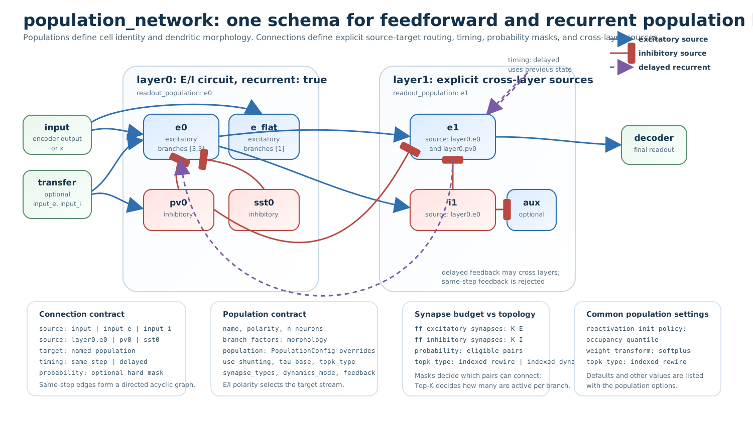
A two-layer population network. layer0 holds two excitatory populations
(e0 with branch_factors: [3, 3] and e_flat with [1]) and two
inhibitory populations (pv0 and sst0); the network input, or the
transfer streams input_e and input_i, drives it. layer1 reads
layer0 populations through qualified sources. Lines ending in an
arrowhead are excitatory connections, lines ending in a bar are inhibitory
connections, and the dashed line is a delayed connection from e1 back to
e0, which requires recurrent: true on layer0. The readout
population of the last layer feeds the decoder. The panels below the
diagram summarize the connection fields, the population fields and how
synapse counts and masks combine; the last panel lists settings that several
examples use, not the defaults.
How a layer computes
Each population has up to four input streams: the same-step streams
ff_excitatory and ff_inhibitory, and the delayed (previous-timestep)
streams rec_excitatory and rec_inhibitory. A connection adds its source
to one stream of its target: the network input and excitatory populations
enter an excitatory stream, inhibitory populations an inhibitory stream. The
sources of a stream are concatenated, and every dendritic compartment of the
target selects a fixed number of synapses from them, set by
ff_excitatory_synapses, ff_inhibitory_synapses,
rec_excitatory_synapses and rec_inhibitory_synapses. The sparse synapse
type (topk_type, see Sparse synapse types) decides how the synapses are
chosen; connection masks decide which source units are eligible.
The populations of a layer run in the order of their same-step connections,
sources before targets. The output of a layer is the output of its readout
population (readout_population, by default the first excitatory
population), and the next layer receives it as input. The network output
is the readout population of the readout layer (readout_layer, by default
the last layer), which feeds the decoder.
When the configuration loads, the structure of the network is checked: every
layer needs an excitatory population, every population needs at least one
enabled same-step connection into its ff_excitatory stream, names must be
unique (population names within their layer) and must not contain a dot, and
connection sources, targets, timing, pathways and probabilities must be valid.
The keys and values of layers, populations, connections and population options
are checked when the model is built, so a misspelled key there fails only at
build time. dendritic-train config.yaml --validate-only builds the model,
datasets and trainer without training and reports these errors early (see
How configs are checked).
Several mechanisms restrict or shape the input of a population. They act at different levels and combine:
Mechanism |
Where it is set |
What it decides |
|---|---|---|
Population |
|
Who the neurons are: polarity, number, morphology and options. |
Connection |
|
Which source may drive which population, in which timestep, and an optional probability mask over source-target pairs. |
Structured connectivity |
|
Masks over individual presynaptic units of a pathway, independent of population names (see Structured connectivity). |
Receptor (synapse) type |
|
How the selected excitatory or inhibitory input is filtered in time (see Receptor synapse types). It does not create a population. |
Soma dynamics |
|
Whether a population emits a rate or spikes (see Spiking soma). |
Connections
Each entry of model.core.population_network.layers[].connections is one
directed connection into a population of that layer:
Field |
Default |
Meaning |
|---|---|---|
|
|
|
|
required |
Name of a population of this layer. |
|
|
|
|
from the source |
Input stream of the target: |
|
|
|
|
|
Probability of each compartment-source pair in a fixed random mask.
|
|
|
Seed of this connection’s mask; overrides the layer’s
|
|
|
Dendritic levels of the target that the connection may contact:
|
A connection whose source, target, timing and pathway repeat an
earlier connection of the layer raises.
External input streams
The first layer reads the network input through three source names:
Without a transfer layer (
use_transfer: false, the default)input,input_eandinput_iare the same tensor.inputandinput_eenter the target’s excitatory stream andinput_iits inhibitory stream, so a population that readsinputandinput_ireceives every input channel as both excitation and inhibition.With
use_transfer: truethe transfer layer turns the input into an excitatory and an inhibitory stream (see TransferLayer).input_eis the excitatory stream andinput_ithe inhibitory stream;inputis the same asinput_e.
input_exc and input_excitatory are accepted for input_e, and
input_inh and input_inhibitory for input_i. input_e and
input_i reach only the first layer, and naming them in a later layer
raises. In a later layer, input is the readout population of the previous
layer, and its synapses take that population’s polarity: an inhibitory readout
population drives ff_inhibitory synapses. External sources cannot use
timing: delayed.
This first layer reads independent excitatory and inhibitory halves of a 784-dimensional input:
model:
  core:
    type: population_network
    population_network:
      input_transform: nonnegative
      use_transfer: true
      transfer_params:
        independent_pathways: true
        excitatory_dim: 392
        inhibitory_dim: 392
      layers:
        - name: layer0
          readout_population: e
          populations:
            - {name: i, polarity: inhibitory, n_neurons: 32, branch_factors: [1]}
            - {name: e, polarity: excitatory, n_neurons: 128, branch_factors: [4, 4]}
          connections:
            - {source: input_e, target: i}
            - {source: input_e, target: e}
            - {source: input_i, target: e}
            - {source: i, target: e}
The input passes through three optional stages before it reaches the first layer, in this order:
input_transformadapts the encoder output:identity(default),nonnegative(checked identity),relu, orsigned_split, which writes the positive and negative parts of each feature as separate non-negative channels and doubles the input width.The transfer layer (
use_transferandtransfer_params).input_projection_dimsadds linear layers, each followed by a ReLU. With a transfer layer they projectinputandinput_eonly;input_ikeeps the width produced by the transfer layer. Setinput_projection_weight_transform: softplusfor positive afferent weights; the defaultidentityretains the historical signed Linear layers. Positive projections check that their inputs are nonnegative and change the model and its initialization (see Biological constraints).
Shunting populations with a positive weight transform treat their input as
non-negative rates. When the first batch shows signed input reaching such a
first-layer population (for example images normalized with
data.processing.normalize: true), the network logs a warning once. Use
input_transform: relu or signed_split, a transfer layer with a
non-negative output_activation, input_projection_dims, or
non-normalized data.
Cross-layer sources
A source of the form layer_name.population_name (a qualified source) reads
a population of another layer. Same-step qualified sources must come from
earlier layers. Delayed qualified sources may come from any other layer,
including later layers, and read that population’s previous-timestep output;
the target layer must set recurrent: true. A qualified source that names
its own layer raises; use the plain population name instead.
In this excerpt of model.core.population_network, the second layer reads
both populations of the first layer instead of only its readout population:
layers:
  - name: layer0
    readout_population: e0
    populations:
      - {name: i0, polarity: inhibitory, n_neurons: 32, branch_factors: [1]}
      - {name: e0, polarity: excitatory, n_neurons: 128, branch_factors: [3, 3, 3]}
    connections:
      - {source: input, target: i0}
      - {source: input, target: e0}
  - name: layer1
    readout_population: e1
    populations:
      - {name: i1, polarity: inhibitory, n_neurons: 16, branch_factors: [1]}
      - {name: e1, polarity: excitatory, n_neurons: 64, branch_factors: [3, 3, 3]}
    connections:
      - {source: layer0.e0, target: i1}
      - {source: layer0.e0, target: e1}
      - {source: layer0.i0, target: e1}
      - {source: i1, target: e1}
Timing
Same-step connections between populations of a layer must form a directed
acyclic graph; a cycle such as i -> e together with e -> i raises when
the configuration loads. Delayed connections (timing: delayed) read the
source’s output from the previous timestep, so they may form cycles, including
a population connected to itself. They require recurrent: true on the
layer, and at the first timestep they read zeros. Mutual E/I interaction is
therefore written as one same-step direction and one delayed direction, or as
two delayed connections.
Pathways and synapse counts
The pathway of a connection is the input stream it feeds. It follows the
polarity of the source unless written explicitly, and it must match the
timing. Each compartment of the target selects <pathway>_synapses contacts
(or the per-level <pathway>_synapses_by_level) from the eligible units of
all sources of that stream. When a mask leaves a compartment fewer eligible
units than this count, the Top-K selection types (standard,
stochastic, variance, dense_to_sparse) use only the eligible ones,
and the indexed types raise.
Every enabled connection must be able to reach a synapse: its pathway needs a
positive count at a depth the connection targets, where the soma counts only
with somatic_synapses: true. The rec_* counts default to 0, so a
delayed connection raises, naming the field, until
rec_excitatory_synapses or rec_inhibitory_synapses is written. A count
written as 0 keeps the connection as a lesion and logs a message. A synapse
count for a stream that no connection feeds is unused.
Probability masks and seeds
probability: p samples, at each dendritic level, a fixed Boolean mask over
the target’s compartments and the source’s units, keeping each pair with
probability p. A compartment left without any eligible unit of a source
receives one unit drawn from that source, so a mask never disconnects a
compartment from a source completely. Synapses are then selected only among
the eligible pairs. Masks are sampled once, when the model is built.
The mask of a connection is seeded by its seed, otherwise by the layer’s
connection_seed, otherwise by 0; dendritic-train fills an unset
connection_seed from experiment.topology_seed (see
Random seeds and reproducibility flags). The seed is offset by the layer, source, target, timing,
pathway, level and shapes, so different connections draw different masks, and
sampling uses its own generator, so it does not change PyTorch’s global random
stream.
With allow_self_recurrence: false, a delayed connection from a population
to itself excludes each neuron’s own output from its compartments.
Dendritic target levels
target_levels restricts a connection to some depths of the target’s
dendritic tree: soma (depth 0), primary (the children of the soma,
depth 1), distal (the outermost level) or explicit depths from the soma.
Synapses at other depths are drawn only from the stream’s other sources. Each
depth that has synapses of a stream must be allowed by at least one of that
stream’s connections; otherwise the build raises. To leave a depth without
synapses, set its count to 0 with *_synapses_by_level. Contacts that
rewiring replaces are drawn within the same restriction. The microcircuit in
Named populations uses target_levels to separate
soma-targeting from dendrite-targeting inhibition.
Connection masks and structured connectivity
The population option structured_connectivity applies a structured mask to
a pathway (see Structured connectivity). A stream can also have a
connection mask, because one of its connections sets probability below 1
or target_levels, or because allow_self_recurrence: false applies to
it. Both masks then restrict the stream: a compartment receives only contacts
that both allow, and a combination that leaves a compartment without any
allowed input raises. Structured rules that place exact contacts
(spatial_morphology and index manifests) cannot also follow a connection
mask, so combining them with one raises.
List-valued probability and indegree of a structured rule are indexed
by the network layer (layers[i]), and each layer draws its own seeded
masks. Layer 0 draws the masks of earlier versions; before 2026-10-11
every layer used the population’s position in its layer for both, so a
population at the same position in each layer read the same list entry and
drew the same mask. Training fills an unset seed of a structured rule from
experiment.topology_seed (since config_version 3; earlier, unseeded masks
drew from the global random stream, which seed: global_rng keeps; see
Structured connectivity).
Named populations
Each entry of model.core.population_network.layers[].populations defines
one named population:
Field |
Default |
Meaning |
|---|---|---|
|
required |
Name used by |
|
|
|
|
required |
Number of neurons (somata). |
|
|
Dendritic morphology, from the soma outward: |
|
|
Population options for this population only (see Options reference). |
population_defaults is merged into every population of the layer, and the
population’s own population block is merged on top of it (nested mappings
such as synapse_types are merged key by key). n_neurons and
branch_factors are set only on the population definition: writing them in
population_defaults or in a population block raises. When a population
sets use_shunting: false and no reactivation_init_policy, it uses
occupancy_quantile (see Gate initialization and maintenance).
Distinct populations can differ in morphology, time constants, synapse counts
and dynamics. A population is a group of neurons, not a receptor mechanism: to
give a population AMPA and NMDA inputs, add receptor types to its options (see
Receptor synapse types) instead of defining a population per receptor.
Populations that differ only in receptor kinetics share their other options
and set different synapse_types blocks in their population overrides.
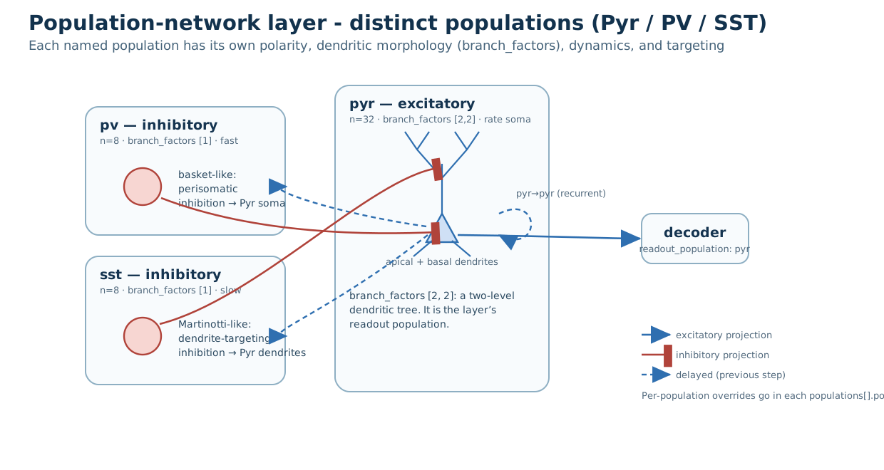
A layer with three populations. pyr is the excitatory readout
population with a two-level dendritic tree; pv and sst are
inhibitory populations with one dendritic compartment per neuron. pv
inhibits the soma and proximal dendrites of pyr, sst its distal
dendrites, and pyr excites itself through a delayed connection. Lines
ending in an arrowhead are excitatory, lines ending in a bar inhibitory, and
the dashed line is delayed. The excitation from pyr to pv and
sst must be delayed, because same-step connections cannot form a cycle.
The configuration below builds this microcircuit. The population blocks
give the three populations different dendritic time constants, and
target_levels separates the two kinds of inhibition:
model:
  core:
    type: population_network
    population_network:
      input_transform: nonnegative
      layers:
        - name: microcircuit
          recurrent: true
          readout_population: pyr
          connection_seed: 123
          population_defaults:
            ff_excitatory_synapses: 12
            ff_inhibitory_synapses: 4
            rec_excitatory_synapses: 8
          populations:
            - name: pyr
              polarity: excitatory
              n_neurons: 32
              branch_factors: [2, 2]
              population: {tau_base: 20.0}
            - name: pv
              polarity: inhibitory
              n_neurons: 8
              branch_factors: [1]
              population: {tau_base: 5.0}
            - name: sst
              polarity: inhibitory
              n_neurons: 8
              branch_factors: [1]
              population: {tau_base: 12.0}
          connections:
            - {source: input, target: pyr}
            - {source: input, target: pv}
            - {source: input, target: sst}
            - {source: pv, target: pyr, probability: 0.45, target_levels: [soma, primary]}
            - {source: sst, target: pyr, probability: 0.25, target_levels: [distal]}
            - {source: pyr, target: pyr, timing: delayed, probability: 0.75}
            - {source: pyr, target: pv, timing: delayed}
            - {source: pyr, target: sst, timing: delayed}
training:
  main:
    strategy: recurrent
The populations pv and sst receive no inhibitory input, so their
ff_inhibitory_synapses count is unused.
Temporal constants and delays
A layer steps through time when it sets recurrent: true, when it has a
delayed connection (which requires recurrent: true), or when one of its
populations uses a temporal feature: a spiking soma, receptor synapse types,
dendritic spikes or soma feedback (see Temporal dynamics). The whole
network then processes sequences [batch, time, features]; a
two-dimensional input is treated as a single timestep. output_mode: mean
or all also makes the network process sequences, with feedforward layers
applied at every timestep.
In a layer that steps through time, every dendritic level l of a population
keeps leaky traces of its raw synaptic currents u (the four input streams
and the input from child branches) and computes its voltage from the traces:
Layers that do not step through time compute the voltage from the currents directly, and the time constants have no effect. Timing has these independent controls:
model.core.population_network.layers[].dtThe integration step \(\Delta t\) of every population in the layer (default 1.0). A delayed connection always reads the previous step.
tau_baseandtau_ratioPer-level time constants when
level_tausis empty: \(\tau_l = \tau_{\text{base}}\, r^{\,n - 1 - l}\) for levelsl = 0(most distal) ton - 1(soma). The soma level usestau_baseand each level further out istau_ratiotimes slower. The defaultstau_base: 50andtau_ratio: 3give[450, 150, 50]for a three-level population;tau_base: 20andtau_ratio: 2give[80, 40, 20].level_tausExplicit time constants, from the most distal level to the soma. The list length must equal the number of levels (
len(branch_factors) + 1).learnable_tauLearns one time constant per level, stored as its logarithm.
connections[].timingdelayedconnections read the source output of the previous step;same_stepconnections read the current step.
Receptor traces (synapse_types), the spiking soma (spike_tau,
spike_readout_tau) and dendritic plateaus (dendritic_spike_plateau_tau)
have their own time constants, which use the same dt; see
Temporal dynamics.
In this excerpt of model.core.population_network, the layer integrates
with a half step, pyr uses geometric time constants [80, 40, 20], and
pv sets and learns its own:
layers:
  - name: circuit
    recurrent: true
    dt: 0.5
    readout_population: pyr
    population_defaults:
      ff_excitatory_synapses: 8
      ff_inhibitory_synapses: 2
      rec_excitatory_synapses: 4
      tau_base: 20.0
      tau_ratio: 2.0
    populations:
      - {name: pyr, polarity: excitatory, n_neurons: 32, branch_factors: [2, 2]}
      - name: pv
        polarity: inhibitory
        n_neurons: 8
        branch_factors: [1]
        population: {level_taus: [5.0, 5.0], learnable_tau: true}
    connections:
      - {source: input, target: pyr}
      - {source: input, target: pv}
      - {source: pv, target: pyr}
      - {source: pyr, target: pyr, timing: delayed}
      - {source: pyr, target: pv, timing: delayed}
Options reference
This section lists every field of a population network: the network fields, the layer fields and the population options. The connection fields are listed under Connections and the population definition fields under Named populations.
Network fields
Fields of model.core.population_network:
Field |
Type |
Default |
Meaning |
|---|---|---|---|
|
list |
required |
Layer definitions, in order (at least one). |
|
int |
encoder output |
Set from the encoder output dimension; a different written value raises. |
|
str |
|
Input adapter: |
|
bool |
|
Split the input into the |
|
mapping |
|
Transfer-layer options (see TransferLayer), including
|
|
list[int] |
|
Widths of linear-plus-ReLU layers applied to the input (to |
|
str |
|
|
|
str or null |
last layer |
Layer whose readout population is the network output. |
|
str or null |
|
Readout population of the readout layer; it must agree with that
layer’s |
|
str |
|
Output of a network that processes sequences: |
|
bool |
|
Record per-level routing information at every timestep of layers that
step through time. |
|
bool |
|
Compile each layer with |
Layer fields
Fields of model.core.population_network.layers[]:
Field |
Type |
Default |
Meaning |
|---|---|---|---|
|
str |
|
Layer name, used by qualified sources and |
|
list |
required |
Population definitions (see Named populations). |
|
list |
|
Connections into this layer (see Connections). |
|
mapping |
|
Population options shared by every population of the layer. |
|
str or null |
first excitatory population |
Population whose output is the layer output. |
|
bool |
|
Step the layer through time and allow delayed connections. |
|
float |
1.0 |
Integration step of the layer (see Temporal constants and delays). |
|
int or null |
|
Seed of the layer’s connection masks; |
|
bool |
|
Record routing information for this layer only. |
Population options
Population options are set in
model.core.population_network.layers[].population_defaults for every
population of a layer, or in layers[].populations[].population for one
population. The tables group them by topic. Several defaults differ from the
corresponding model.core sections of structured E/I cores
(Structured E/I cores): weight_transform defaults to exp here and
to softplus in model.core.morphology, somatic_synapses to true
here and to false there, and reactivation_init_m to 1.0 here and
model.core.reactivation.init_m to 1.5. Write these options explicitly when
results are compared across the two core families.
Synapse counts. Counts are per dendritic compartment. The *_by_level
lists give one count per level, from the most distal level to the soma, and
replace the scalar count when they are not empty.
Field |
Type |
Default |
Meaning |
|---|---|---|---|
|
int |
8 |
Same-step excitatory synapses per compartment. |
|
int |
4 |
Same-step inhibitory synapses per compartment. |
|
int |
0 |
Delayed excitatory synapses per compartment. |
|
int |
0 |
Delayed inhibitory synapses per compartment. |
|
list[int] |
|
Per-level same-step excitatory counts. |
|
list[int] |
|
Per-level same-step inhibitory counts. |
|
list[int] |
|
Per-level delayed excitatory counts. |
|
list[int] |
|
Per-level delayed inhibitory counts. |
|
bool |
|
The soma level receives synapses directly. With |
Integration. See Integration modes for the equations.
Field |
Type |
Default |
Meaning |
|---|---|---|---|
|
bool |
|
Shunting (conductance) integration; |
|
bool |
|
Additive only: normalize the raw additive voltage across the outputs
of each sample. Requires |
|
str |
|
Additive rule: |
|
mapping |
|
Options of a rule registered by a plugin (Additive integration rules). |
|
float or null |
|
Operating-point numerator of |
|
float or null |
|
Operating-point total conductance of |
|
list[float] |
|
Per-depth |
|
list[float] |
|
Per-depth |
|
str |
|
Map from stored parameters to synaptic weights (see Weight transforms). |
|
float |
1.0 |
Leak conductance in the shunting denominator. Values other than 1 require shunting, feedforward rate populations (see Conductance options). |
|
bool |
|
Learn the leak of every compartment; same restrictions as
|
|
str |
|
|
|
float |
1e-8 |
Constant added to voltage denominators for numerical stability. |
|
str |
|
How levels reach the soma: |
|
str |
|
|
Reactivation gates. See Activation functions for the gate functions and Gate initialization and maintenance for the initialization policies.
Field |
Type |
Default |
Meaning |
|---|---|---|---|
|
bool |
|
Apply a reactivation gate to every compartment’s voltage. |
|
str |
|
Gate function. |
|
str |
|
How the gate slope and midpoint start; |
|
float |
1.0 |
Start slope, read only by the |
|
float |
0.5 |
Start midpoint, read only by the |
|
float or null |
|
Lower voltage quantile used by occupancy calibration. |
|
float or null |
|
Upper voltage quantile used by occupancy calibration. |
|
float or null |
|
Gate output targeted at the lower quantile. |
|
float or null |
|
Gate output targeted at the upper quantile. |
|
float |
0.001 |
Smallest voltage spread between the two quantiles that calibration accepts. |
|
float |
50.0 |
Largest calibrated slope. |
|
bool |
|
Keep the previous gate when a calibration is invalid, instead of clamping the fit. |
|
float |
0.25 |
Scale from the robust voltage spread to the slope in the
|
|
str |
|
|
|
bool |
|
Compute |
Initialization. See Synapse initialization for the initializers.
Field |
Type |
Default |
Meaning |
|---|---|---|---|
|
str |
|
Initializer of the dendritic synaptic weights and child couplings. |
|
str |
|
Constructor initializer of the sparse weights; |
|
bool |
|
In the |
|
str |
|
|
|
float |
5.0 |
Total conductance targeted by the adaptive scaling. |
|
float |
1.0 |
Mean child-to-parent coupling at initialization; other values require
|
|
float |
1.0 |
Multiplier of the initial conductances; other values require
|
|
float |
0.0 |
Log-normal spread of the child couplings; positive values require
|
|
int or null |
|
Seed of the population’s initialization streams; |
|
str |
|
Name of the population’s initialization stream; filled as
|
Sparse synapse selection. topk_type selects the sparse synapse type of
every synapse bank of the population; Sparse synapse types lists the types
and their options.
Field |
Type |
Default |
Meaning |
|---|---|---|---|
|
str |
|
Sparse synapse type. |
|
float |
0.0 |
Standard deviation of Gaussian noise added to the selection scores during training. |
|
int or null |
|
Divide each output’s selected weights by their norm of this order. |
|
float |
1.0 |
Scale applied after that normalization. |
|
float |
0.5 |
Noise or sampling temperature of stochastic selection
( |
|
bool |
|
Stochastic selection by noisy Top-K ( |
|
str |
|
Input statistic of |
|
str |
|
|
Indexed synapses. These fields apply to the indexed sparse types
(indexed, indexed_dynamic, indexed_rewire and indexed_release).
See Projection backends for the projection backends.
Field |
Type |
Default |
Meaning |
|---|---|---|---|
|
int or null |
|
Seed of the sampled contacts; |
|
int or null |
|
Candidate pool per output of |
|
str |
|
Selection within the |
|
int |
2048 |
Output rows per chunk of the portable gather; changes memory use only. |
|
int |
100 |
Optimizer steps between |
|
float |
0.05 |
Fraction of each output’s weakest contacts replaced at a rewiring event. |
|
int or null |
|
Last step at which |
|
str |
|
Storage of contact indices: |
|
float or null |
|
Memory budget of the portable gather workspace. |
|
bool |
|
Transform the weights once per recurrent unroll instead of every step. |
|
bool |
|
Another spelling of |
|
bool |
|
Save contact indices in checkpoints; |
|
str |
|
Contact sampling with data parallelism: |
|
str |
|
Projection kernel of indexed synapses. |
Indexed release. These fields apply to topk_type: indexed_release; see
Conductance options.
Field |
Type |
Default |
Meaning |
|---|---|---|---|
|
float |
0.5 |
Lowest release probability. |
|
float |
1.0 |
Highest release probability. |
|
float or null |
|
Weight scale of the release curve
|
|
float |
0.99 |
Decay of the running average of contact impact. |
|
str |
|
Contact impact statistic: |
|
float or null |
|
Optional cap on each effective conductance. |
|
bool |
|
Track presynaptic activity for activity-aware regrowth. |
Dense-to-sparse schedule. These fields apply to
topk_type: dense_to_sparse, which starts with more active synapses and
reduces them to the configured count.
Field |
Type |
Default |
Meaning |
|---|---|---|---|
|
float |
1.0 |
Fraction of candidate inputs active at the start. |
|
int or null |
|
Number of active inputs at the start; replaces the density. |
|
int |
0 |
Step at which the reduction starts. |
|
int |
1000 |
Step at which the target count is reached. |
|
int |
1 |
Steps between updates of the active count. |
|
str |
|
Shape of the reduction: |
|
bool |
|
Keep the active set fixed after the end step. |
|
bool |
|
Advance the schedule once per training forward pass (once per unroll
in recurrent networks); |
|
str |
|
Score that decides which inputs stay active: |
DeepST. These fields apply to topk_type: deepst and credit_deepst;
the credit_* fields apply to credit_deepst only.
Field |
Type |
Default |
Meaning |
|---|---|---|---|
|
float |
0.1 |
Fraction of excitatory inputs connected to each output. |
|
float |
0.1 |
Fraction of inhibitory inputs connected to each output. |
|
bool |
|
Add Gaussian noise to the pruning test. |
|
float |
0.05 |
Standard deviation of that noise. |
|
str |
|
|
|
int |
1 |
Optimizer steps between rewiring events. |
|
int or null |
|
Not read: |
|
bool |
|
Keep the excitatory contacts fixed. |
|
bool |
|
Keep the inhibitory contacts fixed. |
|
str or null |
|
Regrowth initializer; |
|
float |
1e-6 |
Weight at or below which a contact is pruned. |
|
float |
0.95 |
Decay of the gradient trace that scores contacts. |
|
int |
8 |
Inactive candidate contacts observed per branch. |
|
float |
0.1 |
Largest fraction of active contacts replaced per event. |
|
float |
0.5 |
Fraction of weakest active contacts considered for replacement. |
|
int |
5 |
Observations a candidate needs before it can replace a contact. |
|
float |
0.0 |
Predicted improvement a swap must exceed. |
|
bool |
|
Replace contacts even without a predicted improvement. |
|
str |
|
Swap selection: |
|
int |
5 |
Steps of recorded credit before swaps start. |
Connectivity.
Field |
Type |
Default |
Meaning |
|---|---|---|---|
|
mapping |
|
Structured masks of the population’s pathways (see Structured connectivity and the interaction with connection masks above). |
|
int |
position in the layer |
The population’s position in its layer, used in the seed offsets and
index-manifest keys of |
|
int |
index of the layer |
The layer’s index in the network: list-valued options of
|
|
str |
|
Pathway name of the same-step excitatory synapses in
|
|
str |
|
Pathway name of the same-step inhibitory synapses. |
|
str |
|
Pathway name of the delayed excitatory synapses. |
|
str |
|
Pathway name of the delayed inhibitory synapses. |
|
bool |
|
|
Temporal constants. See Temporal constants and delays.
Field |
Type |
Default |
Meaning |
|---|---|---|---|
|
float |
50.0 |
Time constant of the soma level when |
|
float |
3.0 |
Ratio between the time constants of adjacent levels. |
|
list[float] |
|
Explicit time constants, from the most distal level to the soma. |
|
bool |
|
Learn one time constant per level. |
Receptor types and spiking soma. See Receptor synapse types and Spiking soma.
Field |
Type |
Default |
Meaning |
|---|---|---|---|
|
mapping |
|
Receptor types of the excitatory and inhibitory inputs; disabled when empty. |
|
str |
|
Soma output: |
|
float |
1.0 |
Membrane threshold of a spike. |
|
float |
0.0 |
Membrane value after a spike. |
|
float |
20.0 |
Membrane time constant. |
|
int |
0 |
Steps after a spike during which the neuron cannot spike. |
|
float |
10.0 |
Steepness of the surrogate gradient. |
|
str |
|
Population output: |
|
float |
20.0 |
Time constant of the spike trace. |
Dendritic spikes. See Dendritic spikes and plateaus.
Field |
Type |
Default |
Meaning |
|---|---|---|---|
|
bool |
|
Enable dendritic spike or plateau events. |
|
str |
|
|
|
str or list[int] |
|
Levels with events: |
|
float |
0.7 |
Branch voltage that triggers an event. |
|
float |
1.0 |
Amplitude of the plateau’s effect on the branch output. |
|
float |
20.0 |
Time constant of the plateau trace. |
|
int |
0 |
Steps after an event during which the branch cannot fire. |
|
float |
10.0 |
Steepness of the surrogate gradient. |
|
str |
|
How the plateau changes the branch output: |
Soma feedback. See Soma-to-dendrite feedback.
Field |
Type |
Default |
Meaning |
|---|---|---|---|
|
bool |
|
Send the previous step’s soma signal back to dendritic levels. |
|
str |
|
|
|
str |
|
Fed-back signal: |
|
str or list[int] |
|
Receiving levels: |
|
float |
0.1 |
Initial strength of the feedback. |
|
bool |
|
Learn the strength. |
|
bool |
|
One strength per receiving level instead of one shared strength. |
|
float |
0.0 |
Standard deviation of the initial feedback projection; 0 starts it at zero. |
|
float |
1.0 |
Reversal potential of |
Implementation.
Field |
Type |
Default |
Meaning |
|---|---|---|---|
|
bool |
|
Compute the child-to-parent couplings without building the dense block-diagonal matrix (same values, less memory). |
|
str |
|
Gradient scaling of the child-to-parent couplings: |
|
bool |
|
Log the activity of the gradient-scaling hooks. |
The renamed fields topk_strategy, reactivation_strategy and
blocklinear_strategy still load, with a warning, as
topk_gradient_scaling, reactivation_gradient_scaling and
blocklinear_gradient_scaling.
A population that is stepped through time (in a recurrent layer, or with
synapse types, a spiking soma, dendritic spikes or soma feedback) runs each
branch layer once per time step before one backward pass. Its
conductance_dynamic scales are then registered on the tensors of each
step, so every step’s gradients are scaled by that step’s scales; with
topk_gradient_scaling: none only the couplings keep their per-step
tensors. A feedforward population applies the scales of its single forward
pass through backward hooks.
Configuration choices
The table lists common choices, the library default and what to consider.
Choice |
Default |
Recommendation |
|---|---|---|
Integration rule |
|
Set |
Gate initialization |
|
|
Positive conductances |
|
|
Developmental sparsity |
|
|
Multilayer routing |
|
Qualified sources ( |
Recurrence |
feedforward layers |
Set |
Because layer, population and connection keys are checked only when the model
is built, run dendritic-train config.yaml --validate-only after editing a
population network. Sweep axes address population fields by dotted paths with
list indices, for example
model.core.population_network.layers.0.population_defaults.tau_base (see
Parameter sweeps).
Components and code map
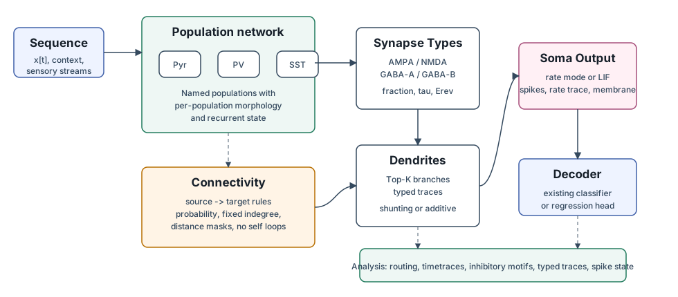
The components that act on a population’s input, in processing order: connections and connectivity masks decide which presynaptic units can contact a population, receptor types filter the selected input, the dendritic tree integrates it with shunting or additive rules, and the soma emits a rate or spikes for the decoder. Analyzers read the intermediate signals.
Configuration |
Implementation |
|---|---|
|
|
|
|
|
|
|
|
|
|
|
Sparse synapse classes registered in
|
|
|
|
|
|
|
|
|
Sequence interface |
The protocols |
All configuration classes above are importable from
dendritic_modeling.networks. Structured and unified E/I cores build the
same StatefulDendriNet populations from their own configuration sections
(see Structured E/I cores).
Examples
configs/examples/population_network_feedforward.yaml is the smallest
complete training configuration of a population network, and
configs/examples/population_network_recurrent_pyr_pv_sst.yaml a recurrent
microcircuit. The table in Example map lists every shipped example,
including multilayer, heterogeneous, CIFAR-10, local-learning and temporal
dynamics configurations.