DendriNet Studio
DendriNet Studio lets you draw a network, inspect the inputs to a neuron, train the model and compare runs in a browser on your computer. The editor and the command line use the same experiment YAML and the same DendriNet model builders and trainer. You can move a design between them at any point.
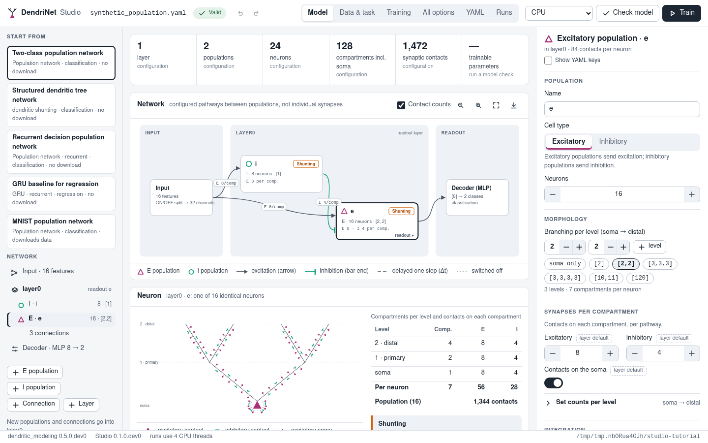
The Model view of the two-class tutorial. Excitatory populations are triangles and send arrows; inhibitory populations are circles and send bars. The neuron below the network is the selected population’s exact compartment tree with its contacts per compartment.
Install and start
In a fresh Python 3.10 or later environment on your computer, install Studio from PyPI. Pip installs the compatible core library and PyTorch.
python -m pip install dendrinet-studio==0.1.0
dendrinet-studio --workspace my-runs
For an editable install, run python -m pip install -e . -e ./apps/studio
from the repository root. See Installation for environment setup.
The command opens the local app and prints its address. If the tab fails to
open, paste the whole printed address into a browser on the same computer,
including its port and the session token after #. Keep the command running
while you work. Ctrl+C stops the server and its workers. Training takes place
on the computer running the command. A local installation works offline after
its dependencies and any required datasets have been downloaded.
Option |
Meaning |
|---|---|
|
Folder for run records and results (default |
|
Local port (default 8765; the next free port when it is taken; 0 picks any free port). |
|
CPU threads per run (default: up to 4, depending on the computer). |
|
Print the address without opening a browser, for remote machines. |
|
Design and export only: Studio never builds or trains a model on this
machine (also set by |
|
Also accept requests addressed to |
On a remote machine (a workstation or a cluster compute node), start Studio
with --no-browser, forward its port from your computer and open the
printed address locally:
# on the remote machine
dendrinet-studio --workspace ~/studio-runs --no-browser
# on your computer
ssh -L 8765:127.0.0.1:8765 user@remote-host
Use the actual port printed by Studio on both sides of the tunnel. If a scheduler assigned a compute node, the tunnel must reach the machine running Studio. A new session prints a new token.
Train your first network
In Model, open the two-class population example under Start from (
synthetic_population.yaml). It generates its own data. Select populatione. Its 16 excitatory neurons each have two branches leaving the soma and two children per branch. The eight inhibitory neurons in populationireceive excitation from the input and supply inhibition toe.Select CPU, then Check model. When the worker finishes, open its entry under Runs → Model checks. The model check reports trainable parameters, active synapses and candidate connections. Editing the design and checking it again creates a separate record.
Under Training, set Epochs to 1 for a quick test. Choose Train, name the run and select Start training. In Runs, open the finished training entry to inspect its loss, available evaluation measures and log.
For a comparison, change the epoch count, keeping the seed and network fixed, and train a second time. Select the two runs using their checkboxes. The comparison shows both learning curves and the settings that differ.
In YAML, choose Export to save the design. If you save the file as
demo.yaml, you can run it in the same environment withdendritic-train demo.yaml. To get the original, unedited example directly, usedendritic-example synthetic_population --output original.yaml.
Trace excitation and inhibition into a neuron
Select a first-layer population in Model. Its polarity describes the synapses it sends. Synapse sources per neuron shows the inputs it receives. In the two-class tutorial, external excitation drives both populations. The excitatory neurons receive their inhibitory contacts from the local inhibitory neurons. In a design with direct external inhibition, the table names the external inhibitory stream instead.
Desired input to the selected population |
Settings in External input to this population |
|---|---|
External excitation with inhibition supplied locally |
Enable Direct external E. Leave Direct external I off. Connect the local I population to the target and set its incoming I contact budget. |
Both signs supplied by the input |
Enable both switches and give both pathways contacts. For a biological model, choose Distinct E and I afferents with matched features or Separate groups of input channels under External afferents for the first layer. |
Only inhibition supplied by the external input |
Connect a same-step excitatory population first. Enable Direct external I and turn off Direct external E. Each target needs a same-step excitatory source. |
The switches edit connections to the selected target. The external afferent
choice applies to the whole first layer. In YAML, input or input_e
supplies excitation and input_i supplies inhibition. With transfer
enabled, input_source_identity: paired_afferents gives distinct E and I
afferents the same feature values. With independent_pathways: true, the
two streams read separate groups of channels. ON/OFF encoding
(input_transform: signed_split) is a separate choice about how to encode
feature values. In later layers, input refers to the preceding layer’s
readout. See Population networks for connection and transfer settings.
Under Synapses, set counts per compartment or use Set counts per level. Depth 0 is the soma. The level table gives the count on one compartment. The source table sums the budget over one neuron. Two sources on the same pathway share that budget. Enabling an additional source does not double it.
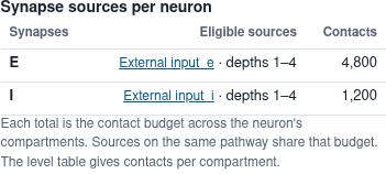
In the empirical CIFAR-10 example, 120 dendritic compartments each receive
40 E and 10 I contacts. The corresponding totals are 4,800 and 1,200 per
neuron. Both external populations carry matched features. To inspect this
design from the repository, import
projects/empirical/configs/cifar_primary_shunting.yaml in the YAML view.
The study’s README gives the library version used for its published runs.
For structured feedforward E/I cores, First-layer feedforward sources lists the routes fixed by the architecture. Local I cells, when present, supply the E cells’ inhibitory input. Without local I cells the first-layer E cells can receive the external I stream directly. Change counts under Connectivity, population sizes under Architecture, and external channel identity under Transfer.
What Studio supports
Model family |
How it is edited |
|---|---|
|
Visually: layers, excitatory and inhibitory populations, neuron counts, dendritic morphology (branching per level), contacts per compartment for each pathway (one count or one per level), contacts on the soma, the integration rule (shunting or the additive rules), leak, dendritic gates, initialization, time constants and every other population option; connections between populations with their timing (same step or delayed by one step), pathway, target levels, probability and seed. |
Structured dendritic trees ( |
Forms for the architecture, connectivity, morphology, transfer, sparsity, gate and implementation sections. |
Recurrent baselines ( |
Typed forms for the family’s options. |
Other built-in core types |
Forms where the library types the section; YAML for nested options. |
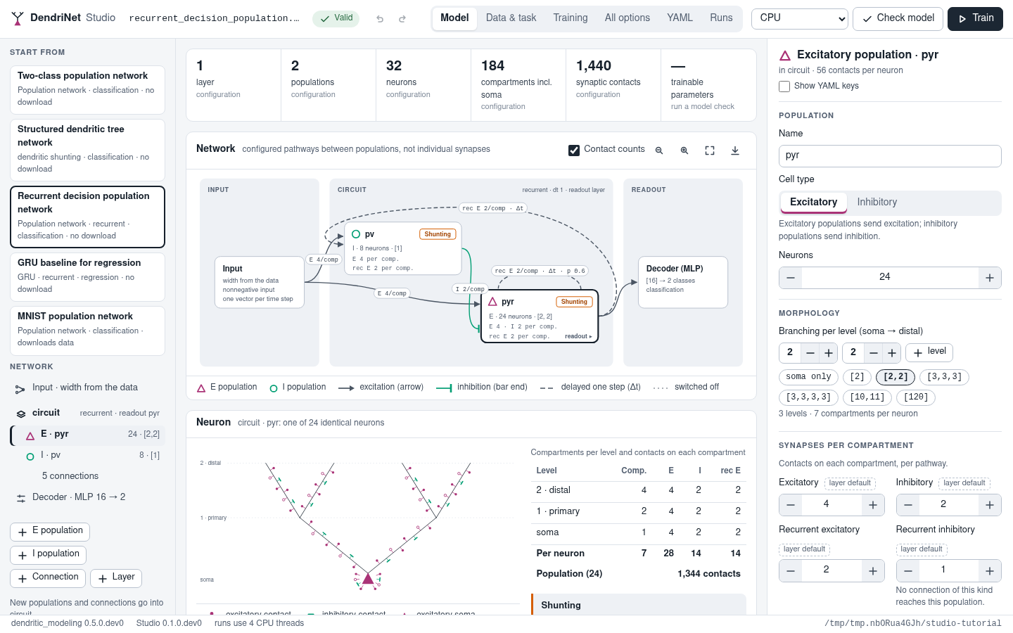
The recurrent decision example. Delayed connections (dashed, Δt) carry the previous time step’s activity, which makes the layer recurrent.
For every family Studio edits the task (classification or regression), the dataset and its options, the loss (only losses that suit the task are offered first), the learning strategy (standard backpropagation, recurrent training, the local learning rules and the staged strategies), the optimizer, learning rates per parameter group, the schedule, early stopping, initialization (synaptic weights, branch couplings and gates), seeds, regularization, pruning and evaluation measures. Values the forms do not show are kept: the All options view lists every option of the configuration with a search box, and the YAML view edits the file directly.
The installed examples cover each kind of model:
Example |
What it shows |
|---|---|
|
A feedforward E/I population network on a generated two-class task. It defaults to 30 epochs and runs locally without a dataset download. |
|
The same task with the structured dendritic tree family. |
|
A recurrent population network with delayed recurrent connections on a context-dependent evidence-integration task (classification over time). |
|
A GRU baseline on the adding problem, a regression task over a sequence. |
|
The tutorial’s network on MNIST digits; the first run downloads MNIST. |
Export any of them without Studio with
dendritic-example <name> --output my_model.yaml.
Working in Studio
The tabs at the top hold the views of one design. Check model and Train work on the design as it is; the status next to the file name says whether DendriNet accepts it (a word and an icon, never a colour alone).
Model. Pick an example on the left or keep editing the current design. Select a population, a connection (click its line or its label) or a layer lane to edit it on the right. A tag such as layer default marks values that come from a default; reset removes a setting so the default applies again. To extend a population network:
Select the receiving layer and choose E population or I population. Set the neuron count and the branching factors from the soma outward. For example,
[2, 2]gives two proximal and four distal compartments per cell. The soma only preset gives a point neuron. Use Contacts on the soma when the design calls for direct somatic input.Use Connection to choose a source and target. Set whether the connection carries current-step or previous-step activity and which target depths receive it. Use Synapses on the receiving population for the corresponding feedforward or recurrent E or I contact count.
Use Layer to extend the stack. Select a layer to choose its readout population. The next layer receives that population’s output. Select the network to choose which layer supplies the decoder.
An invalid edit is reported and the drawing keeps the last valid preview. Small neurons are drawn in full when their branches fit. For large trees, the neuron view draws representative branches and labels how many children each represents. The caption gives the number drawn and the total, including the soma. The adjacent table covers every configured depth. Use undo and redo (Ctrl+Z, Ctrl+Shift+Z) to revisit a design, and Show YAML keys to see what a field writes. The diagram can be zoomed, fitted to the panel and exported as SVG.
Data & task. The task, the number of classes or outputs, the loss, the dataset (grouped into generated data, sequence tasks and image datasets that download once into the data cache) and its options, splits, seeds and evaluation measures.
Training. The learning strategy and its options, the schedule, the optimizer and the learning rate of each parameter group, initialization and seeds, dendritic gate calibration, regularization and pruning, and data loading and precision settings. For population networks, initialization settings apply to every layer; a layer or population can still override them.
All options. Every section of the configuration with a search box.
YAML. Edit the design and choose Apply (Ctrl+Enter). The strict
loader checks it before replacing the current design. If you continue typing
during validation, choose Apply again to use the latest text. Restoring
an unsaved design keeps its browser draft available across reloads. Syntax errors include
the line when the parser can identify it. Import opens a standalone
experiment. Export writes its settings as YAML. Re-exporting preserves
configuration values, including options without a graphical control.
Comments and original formatting are lost. For a sweep, use
dendritic-sweep --config my_sweep.yaml --generate-only and import one
generated experiment. For a file that uses extends, open an already
composed experiment with its parent settings included. See Composing configs with extends
and Parameter sweeps.
Runs. Every model check and training run in the workspace. Running trainings show their progress. Select up to eight training runs to overlay their loss curves. Each run has its own marker shape and a text label. The view compares final measures in a dot plot and a table and lists settings that differ. Select a run to see its status, timing, model size, command, folder, notes and worker log. Open in editor loads its configuration back into the design. The curves can be exported as CSV.
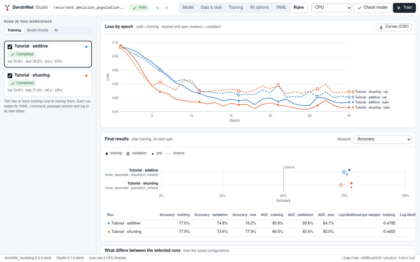
Two runs of the tutorial compared in the Runs view.
Model checks, previews and runs
The preview that redraws the design after every edit validates the configuration and resolves the population graph; it does not build weights, download data or touch a random stream. A population card shows the contact budget for each input stream. When several connections supply the same stream, the card labels their combined budget as shared. The connections show their polarity and any target-level restrictions. Checking the model reports the active contact count after construction.
Check model builds the network in a separate process with the dataset’s input shape and the configured seeds, and reports trainable parameters, active synapses and candidate slots, before gate calibration. The selected dataset is prepared first, so a check of an image dataset may download it.
Train calls the same Python entry point as dendritic-train. The
device selector offers CPU or GPU if available. One check or training
worker runs at a time. Studio writes each run in its own workspace folder.
For instance, a training run with the tutorial defaults produces:
my-runs/20261118-142713-1f56b0/
  config.yaml        # the design as submitted
  studio_run.json    # config hash, command, device, threads, core path and version
  worker.log         # everything the worker printed
  results/model_*/   # the library's normal run outputs and records
Studio passes --output_dir <run-folder>/results --run_name model to the
trainer. The name entered in the browser labels the Studio record. Use the
saved command, working directory and device settings to reproduce the
launch. Set an absolute data.base_dir when several runs should share a
local dataset. For a check, the resource counts live in resources.json.
For training, see Runs and outputs for the trainer’s configuration,
seeds, metrics and environment records.
A run is reported as completed only when its worker exits successfully. A run
that was active when Studio stopped is shown as unknown, never as completed.
Studio runs one process on this machine; distributed training and cluster
submission stay with dendritic-train, torchrun and dendritic-sweep,
which read the exported YAML.
Troubleshooting
Browser says the site cannot be reached. Confirm the command is still running and use its printed port. A browser on another computer needs a connection to that host (see Install and start). If the page opens but cannot reach the local service, reopen the complete URL with its current token.
The diagram looks valid but Check model fails. The live preview validates the configuration. The check also constructs the model with a sample from the configured dataset. Open Runs → Model checks, select the failed check and read Worker log for the loader or constructor error.
The controls for starting a run are missing or disabled. A design only label means the server was launched with execution disabled. With execution enabled, clear any field error and finish or stop the current worker.
Privacy and security
Studio listens on the loopback interface only. Its programming interface requires the session token and an accepted host name. Treat the printed URL as private. The browser interface loads its assets locally and has no telemetry. A dataset loader can contact its data provider when a configured dataset needs downloading. The server and its workspace are intended for one user.
Accessibility
Meaning never rests on colour alone: excitatory and inhibitory populations differ by shape (triangle, circle) and by line ends (arrow, bar), delayed connections are dashed, statuses carry an icon and a word, and every run in a comparison has its own marker shape and a text label. Alt+1 to Alt+6 switch views. Use the labelled population and connection buttons in the outline to select elements with the keyboard. Light and dark themes follow the operating system.
For developers
Studio lives in apps/studio of the DendriNet repository and is built as
its own wheel. The server (dendrinet_studio.server) is the Python
standard library’s HTTP server; the client is plain HTML, CSS and JavaScript
modules with no build step and no external requests.
Module |
Role |
|---|---|
|
Describes every configuration section, option, type, default and allowed value, read from the library’s dataclasses and registries. |
|
Validates a configuration with the library’s strict loader and describes it for the editor (population graph, per-level contacts). |
|
Starts, stops and records worker processes and reads their results. |
|
The model check: builds the model as the trainer does and writes its resource counts. |
|
The client: |
Run the tests on a workstation or compute node:
PYTHONPATH=src:apps/studio/src python -m pytest apps/studio/tests -m "not slow"
PYTHONPATH=src:apps/studio/src python -m pytest apps/studio/tests
The slow tests build and train small models, and the browser tests drive
Chromium through Playwright (pip install -e "apps/studio[test]" and
python -m playwright install chromium); they are skipped when Playwright
is missing. Set STUDIO_BROWSER_ARTIFACTS=<folder> to keep their
screenshots.